A field built from atoms, energy, and models. Computational materials science studies how the arrangement and interaction of atoms give rise to the properties of a material. Rather than treating a material as a black box, it asks which atomic configurations are stable, how energy changes with composition and temperature, and how those changes shape phase behaviour, diffusion, and processing.
Computation does not replace experiment. It helps explain experiments, compare hypotheses that are difficult to isolate in the laboratory, and explore compositions before they are made.
Scope. UEM and UEM–Miedema apply only to solution phases (melts and disordered solutions). They are not used for crystalline solids; those require DFT/AIMD.
Many useful materials are solutions of three or more components. Their behaviour is governed by the Gibbs energy of mixing, and especially by its excess part: the departure from ideal mixing caused by interactions between unlike atoms. From the excess Gibbs energy come activities, chemical potentials, and the interaction coefficients that describe how one solute changes the behaviour of another.
The difficulty is practical as well as conceptual. Binary data are comparatively plentiful, while complete measurements for every ternary, quaternary, and higher-order combination are costly and sometimes impossible. A reliable method is therefore needed to estimate multicomponent properties from binary information, without pretending that the higher-order system is merely a sum of unrelated pairs.
UEM unifies traditional geometric models (Kohler, Muggianu, Toop, and related models) in a single expression. Instead of choosing one classical rule in advance, UEM uses contribution coefficients, determined by differences in properties between components, to decide how strongly each binary contribution enters the multicomponent estimate.
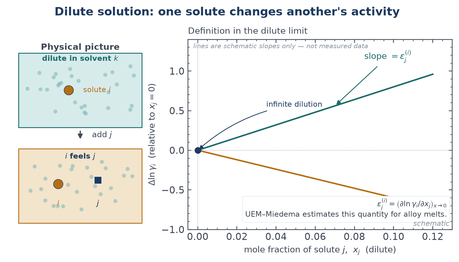
When binary Redlich–Kister data are available, prefer activity interaction coefficients ε obtained from those binary parameters. When binary data are unavailable, UEM coupled with Miedema mixing enthalpies and excess-entropy relations can estimate dilute solute–solute ε in alloy melts — how one solute changes the activity of another when both are present in small amounts.
The same framework is presented here as knowledge and as a working tool. The UEM page explains the problem and the unifying idea, the Knowledge page supplies supporting methods (molecular dynamics, density functional theory, and quantum mechanics for computation), and the Calculators page lets readers try the dilute-solution and binary-extrapolation calculations in the browser.
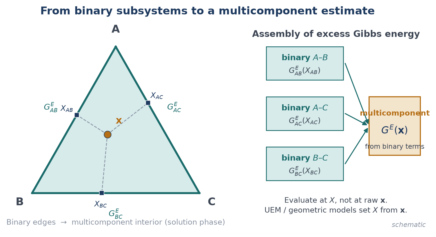
UEM generalises classical geometric extrapolation by replacing fixed, composition-independent weighting with a contribution coefficient α. For a multicomponent solution, the excess Gibbs energy is assembled from its constituent binary sub-systems. Symbols: in the dilute Wagner definitions (formulas 1–3), i and j are solutes and k is the solvent in a ternary k-i-j system; in the geometric and UEM formulas (4–7), i, j, and k are general components. x is mole fraction, R is the gas constant, T is temperature, GE is excess Gibbs free energy, γ is the activity coefficient, and ε is the activity interaction parameter.
It shows how solute j changes the activity coefficient of solute i in the dilute limit.
It links the activity coefficient to excess Gibbs free energy.
If the ternary excess Gibbs free energy is known, ε follows by differentiation in the dilute limit.
The ternary excess property is built from its three binary terms, evaluated at sub-binary compositions X that depend on the extrapolation model.
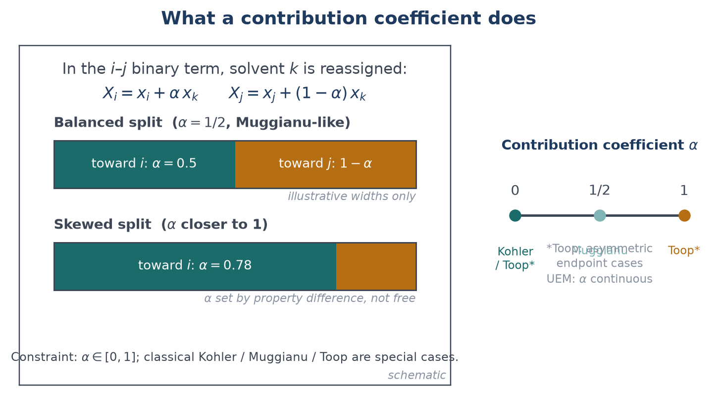
αi(ij)k is the UEM contribution coefficient: the share of component k assigned to component i in the i-j sub-binary term. It is determined by property differences between components, which is what unifies the traditional geometric models in one expression. Contribution coefficients satisfy α ∈ [0, 1] and αi + αj ≤ 1.
D measures how different component k is from component i, through its partial molar excess property in the relevant binary systems. A larger D means a larger property difference.
The binary excess Gibbs free energy splits into excess enthalpy (from assessed binary data or, when those are missing, from the Miedema model) and excess entropy terms.
Classical geometric models emerge as special, composition-independent limits of α — Kohler (α = 0), Muggianu (α = 0.5), Toop (α in {0, 1}, asymmetric) — while UEM lets α respond continuously to the underlying thermodynamic data.
This section deliberately does not present measured performance plots for any specific alloy system. The figures below are original schematics that explain how the framework works. They contain no measured values, no fitted results, and no system-specific performance data. Readers who want the published record should use the Publications page.
The UEM and UEM–Miedema calculations described above are available as browser calculators on this site. No software is installed and no data are sent to a server: the calculations run in the visitor's browser.
Only the verified papers that support the account of UEM given on this site are listed. Each entry gives the title, journal, year, volume and pages, and a DOI link only where a DOI was verified for this list.
Readers who want the main idea first can start with UEM and its progress, which moves from the geometric-model problem to the unified expression and its applications in dilute solutions. Readers who want the methods behind the idea can turn to molecular dynamics, density functional theory, and quantum mechanics for computation, each presented through its concepts, key ideas, and reasons for caring about it. Applications are kept general and tied to published work; this site does not present unpublished research details, numerical results, or proposal material.